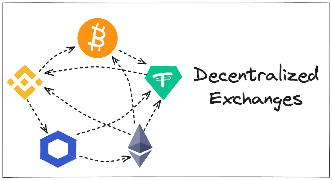
In the midst of the COVID lockdown, my curiosity about the financial markets soared. The infamous GameStop incident on Robinhood[1] piqued my interest in understanding the dynamics of trading from a different perspective. In the course of this exploration, I discovered decentralized finance (DeFi). The censorship and limitations of traditional financial systems made the potential of a permissionless and decentralized financial landscape even more appealing. While the initial DeFi buzz may have faded, the demand for an uncensored, permissionless, and fair financial system is stronger than ever.
Table of Contents
- What is a Decentralized Exchange?
- Order Book Based DEXs (Relayer Model)
- A Simpler Way to Build a DEX?
- Uniswap
- Marginal Price & Slippage
- Incentives for Liquidity Providers
- Limitations of Uniswap V2: Capital Efficiency
What is a Decentralized Exchange?
Let's briefly explore the concept of decentralization and decentralized exchanges. Being decentralized simply means there's no central authority or controlling party. For example, Bitcoin doesn't have a CEO of Bitcoin or the Bitcoin Government.
So, what is a decentralized exchange? Here's a definition from Coinbase:
A decentralized exchange (or DEX) is a peer-to-peer marketplace where transactions occur directly between crypto traders. DEXs fulfill one of crypto's core possibilities: fostering financial transactions that aren't officiated by banks, brokers, or any other intermediary. Many popular DEXs, like Uniswap and Sushiwap, run on the Ethereum blockchain. [2]
As Coinbase highlights, DEXs eliminate the need for intermediaries like traditional finance. Customer funds aren't held in a centralized account; DEXs can't manage user's funds at all. Instead, funds are held in transparent smart contracts that anyone can verify. This arrangement prevents incidents like the FTX implosion. Revenue generated from trading fee is shared with liquidity providers (LPs), but unlike in traditional finance, the barrier to becoming an LP is virtually nonexistent. Anyone can be an LP and share in DEXs' revenues.
NASDAQ's annual revenue for 2022 was $6.226B[3]. As a stock exchange, a significant portion of its income comes from transaction fees. I'm not suggesting DEXs will match NASDAQ's size one day, but they do allow ordinary people like me to share in revenue from transaction fees. Anyone can be an LP on DEXs. Anyone can list their tokens on DEXs and no single entity owns or controls the exchange. Can you see why I find DEXs so fascinating?
In this article, I'll delve into the mechanics of decentralized exchanges (DEXs) and explain their inner workings.
Order Book Based DEXs (Relayer Model)
The initial approach to building a DEX was the order book model, which matches orders from buyers and sellers based on a set of rules. It's widely used in popular stock exchanges, foreign exchanges, and other markets with sufficient liquidity.
In the early days, a centralized "Relayer" performed the matching off-chain. This relayer created an off-chain transaction resembling an atomic swap and submitted it to the blockchain for on-chain settlement. Here are a few examples of DEXs that initially adopted this model:
However, most DEXs have moved away from this model due to its limitations, which include composability, dependency on a centralized party, difficulty in bootstrapping liquidity, and high costs associated with today's blockchains because of gas. Here is an article by Will Warren that explains the limitations of the order book model: Front-running, Griefing and the Perils of Virtual Settlement
A Simpler Way to Build a DEX?
To overcome these limitations, DEXs have shifted to the Automated Market Makers (AMMs) model. AMM enables efficient trading, even with thin liquidity.
A Brief History on Automated Market Makers.
The idea of AMM was proposed by Vitalik Buterin in a 2016 Reddit post. Before AMMs, prediction markets used Hanson's Logarithmic Market Scoring Rules to price shares, which is a method also used in online ad pricing. Following Vitalik's proposal, Alan Lu and Martin Koppelman generalized the AMM model. For more on this, see their blog post Building a Decentralized Exchange in Ethereum and Alan's conference talk, Making Predictions Conditionally by Alan Lu of Gnosis
Smart Contracts as AMMs
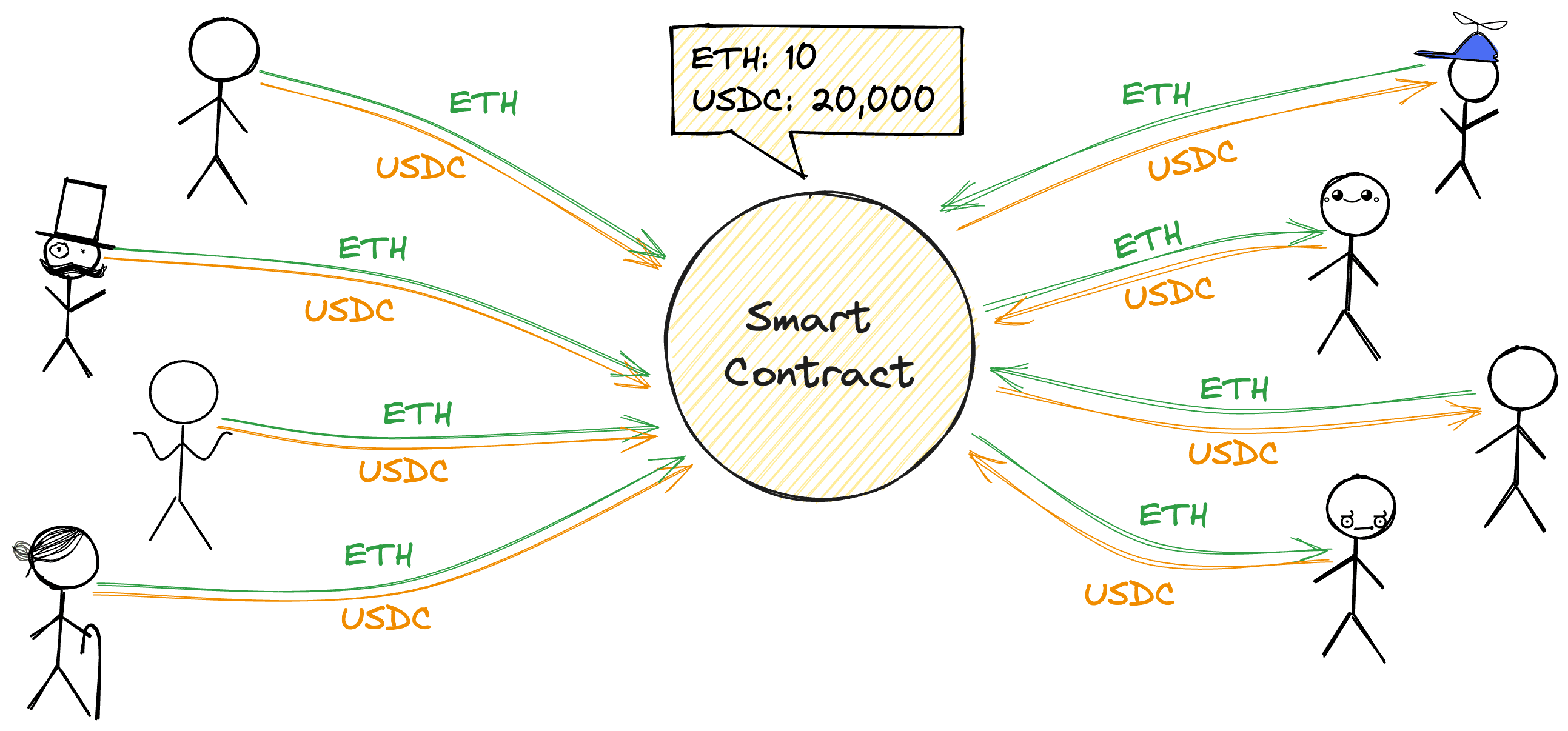
How does a smart contract work as an AMM? It maintains the invariant that for some constant (in the version where people can invest, can change, but only during investment/withdrawal transactions, NOT trades). Anyone can buy or sell by selecting a new point on the curve, supplying the missing A tokens, and in exchange, receiving the extra B tokens (or vice versa). The "marginal price" is simply the implicit derivative of the curve, or .
Here is an example:
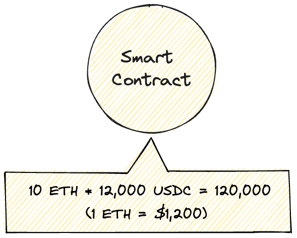
Our AMM smart contract is holding 10 ETH and 12,000 USDC. Here our is 10.0, is 12,000 so becomes 120,000. Currently, the price of ETH is $1,200 in our pool.
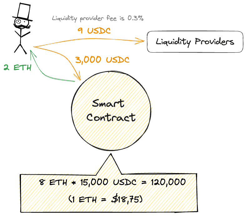
Now, you want to swap your USDC for ETH. If you sell 3,000 USDC to the AMM, how much ETH will you get? First, divide by the new supply of USDC in the pool, which is ETH. , so you will get 2.0 ETH from your 3,000 USDC.
However, in the example above, we disregarded the fee we pay to the LP (liquidity providers). If we assume the fee to the LP is 0.3%, you will have to pay about 9.0 USDC as a fee. As a result, you will need to pay 3,009 USDC to get 2.0 ETH.
If we look at the curve, it looks like below:
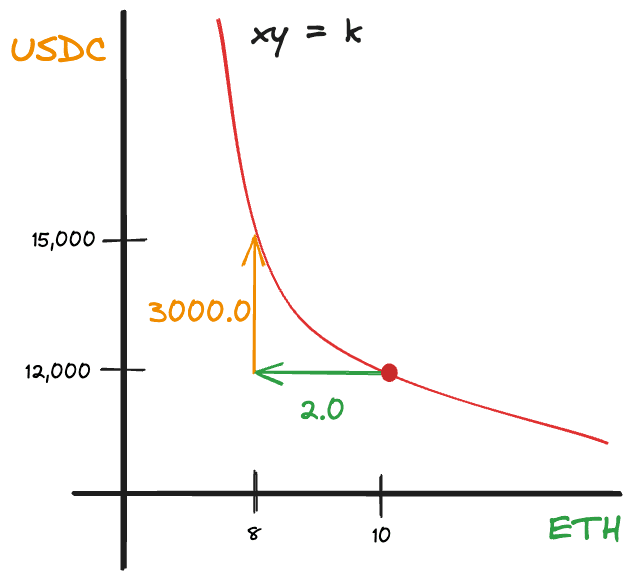
Pretty simple, right? By selling 3,000 USDC, you moved from (10.0, 12,000) to (8.0, 15,000) on the curve.
Uniswap
Let's learn more about DEXs by looking at the most successful DEX: Uniswap.
Uniswap v2's Pricing rule
Uniswap V2's pricing rule is:
where is the percentage fee that is paid to liquidity providers, and where and .
This rule specifies the price of buying in terms of .
A similar exercise (swapping s and s) produces a rule that specifies the price of selling in terms of :
Here's an example where the contract contains 4.0 ETH and 2000.0 USDC and charges a fee for liquidity providers of 30 bps:
Suppose Alice wants to sell 8.0 ETH to the contract. How much USDC should she get in return?
(The fee to liquidity providers is 6 USDC and 0.024 ETH.)
Real life example
We can see the pricing rules used in Uniswap V2's code.
Selling for
// given an input amount of an asset and pair reserves, returns the maximum output amount of the other asset
function getAmountOut(uint amountIn, uint reserveIn, uint reserveOut) internal pure returns (uint amountOut) {
    require(amountIn > 0, 'UniswapV2Library: INSUFFICIENT_INPUT_AMOUNT');
    require(reserveIn > 0 && reserveOut > 0, 'UniswapV2Library: INSUFFICIENT_LIQUIDITY');
    uint amountInWithFee = amountIn.mul(997);
    uint numerator = amountInWithFee.mul(reserveOut);
    uint denominator = reserveIn.mul(1000).add(amountInWithFee);
    amountOut = numerator / denominator;
}
Buying for
// given an output amount of an asset and pair reserves, returns a required input amount of the other asset
function getAmountIn(uint amountOut, uint reserveIn, uint reserveOut) internal pure returns (uint amountIn) {
    require(amountOut > 0, 'UniswapV2Library: INSUFFICIENT_OUTPUT_AMOUNT');
    require(reserveIn > 0 && reserveOut > 0, 'UniswapV2Library: INSUFFICIENT_LIQUIDITY');
    uint numerator = reserveIn.mul(amountOut).mul(1000);
    uint denominator = reserveOut.sub(amountOut).mul(997);
    amountIn = (numerator / denominator).add(1);
}
Marginal Price & Slippage
The price of a token is the ratio between the amount of one asset (like USDC) paid and the other asset (like ETH) received. For example, if you pay 1000 USDC to receive 4 ETH, then the price of each ETH is 250 USDC. In our notation, this is given by .
Observation #1
The price depends on the size of the trade,
Consider an example where 20.0 ETH * 6.0 USDC = 120.
- Buying 10 ETH (i.e costs 6.02 USDC or 0.602 USDC per ETH.
- In contrast, buying 5 ETH costs 2.006 USDC or 0.401 USDC per ETH.
When approaches 0:
If we set the fee to zero , then:
equals the magnitude of the slope of the tangent line.
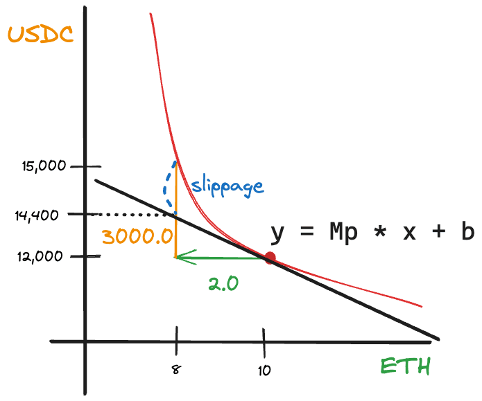
As depicted in the graph above, your slippage increases with .
Observation #2
Pricing also depends on the size of x and y, or in other words, on k.
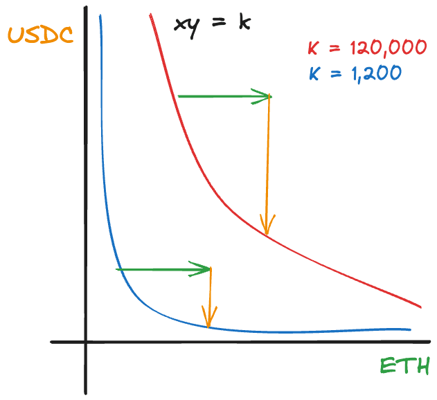
It's evident that as k increases, the effective price of the AMM becomes less sensitive to .
Incentives for Liquidity Providers
Let's explore the incentives for liquidity providers.
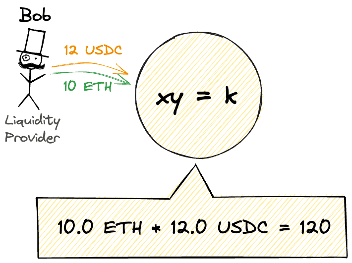
Consider an example where Bob deposits 10 ETH and 12 USDC of liquidity, which implies:
Bob waits for a month, during which traders drive $700 worth of volume through Bob's AMM pool. At the end of the month, Bob withdraws his ETH and USDC. By this time, the price of ETH has gone up 4x. The marginal price is now:
Assuming , what is Bob's return?
First, what does Bob earn from the trading fee?
Second, how much ETH and USDC does Bob get back?
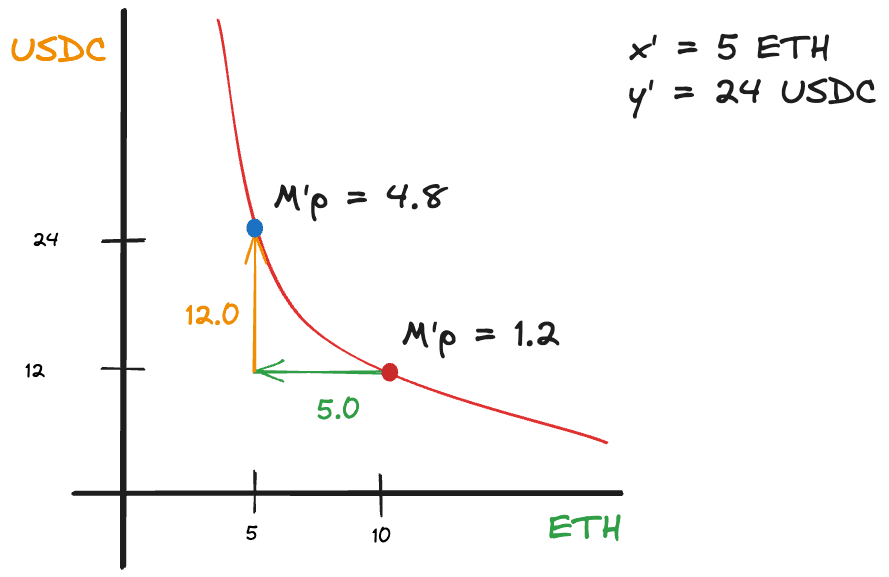
Bob gets back 5 ETH and 24 USDC. So, Bob's total return is: 5 ETH and 26.1 USDC.
Divergence Loss
So, how did Bob do?
Measured in USDC, Bob now has:
50.1 USDC is not bad, but how would he have done if he had just held on to his 12 ETH and 10 USDC?
He would have earned more if he had simply held on to his ETH and USDC. This is referred to as impermanent divergence loss. It is divergence because Bob's return diverged from his baseline return . The usual term is impermanent loss, but I prefer to call it divergence loss because it is more descriptive.
What if volume had been higher?
Say, the volume had been 10x higher: 700.
Therefore,
This time, Bob's return is higher than his baseline return of 67.6 USDC. His profit is:
Trading volume had to be higher for Bob to make a profit.
Calculating Profit
Bob's return is given by:
His baseline return is given by:
Therefore, his profit in percentage terms is given by:
Let's ignore the volume term for now, and simplify:
Recall from our curve that . Thus, and . Also, and . Finally, let:
Now we can simplify our profit equation:
Step 1: Let's express everything in terms of and .
Step 2: Reintroduce the volume term.
Step 3: Plot this equation.
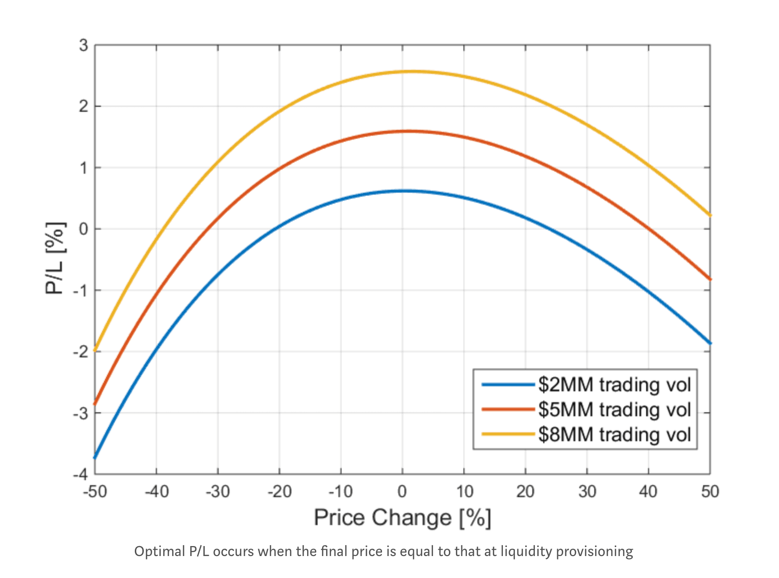
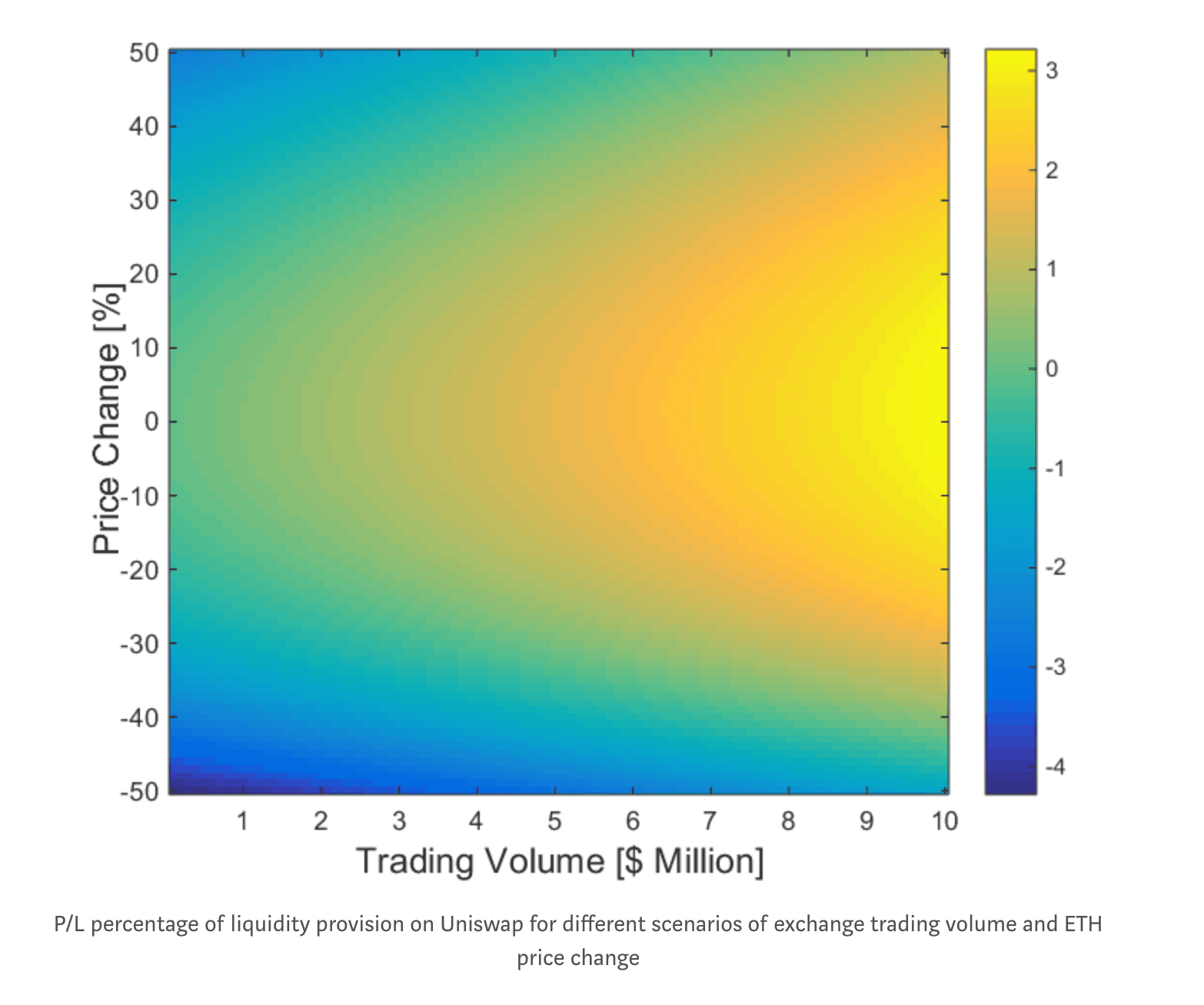
As you can see, the profit is maximized when the price is equal to that at which the liquidity was provided. And of course, more volume means more profit.
What if Bob wants to supply liquidity to only that middle section of the curve where the price is almost equal to the price at which he provided liquidity? That's where Uniswap V3 comes in.
Limitations of Uniswap V2: Capital Efficiency
Uniswap V2 has a major limitation: it requires you to provide liquidity for all price range. What do I mean by that? Take a look at the curve again:
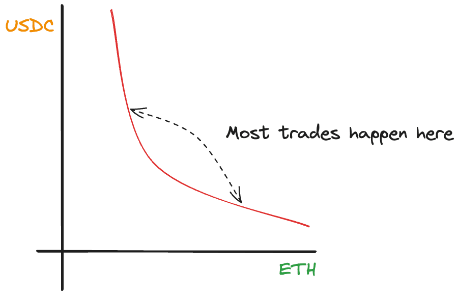
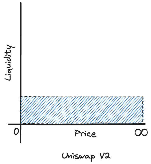
Even though most of the trading volume happens around the current price, you still need to provide liquidity for the entire price range.
One approach to solve this issue is: Curve Finance. Curve Finance is a decentralized exchange that is optimized for stablecoins. Unlike UniSwap V2, Curve's curve looks like this:
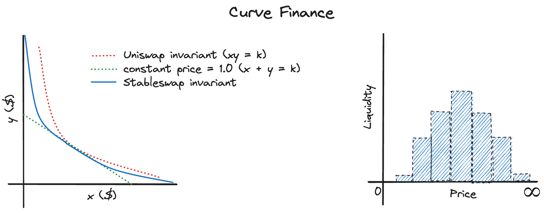
As you can see, Curve's curve is much flatter than UniSwap V2's curve. This means that Curve is much more capital efficient than UniSwap V2. I would love to discuss more about Curve's stable swap mechanism, but it deserves another article. If you are interested, you can read more about it here.
Uniswap V3
Uniswap V3 addresses the capital efficiency issue by enabling liquidity providers to allocate liquidity within a specific price range. For more information, check out this video from the Uniswap team:
If you've read this far, you should have a solid understanding of how Uniswap operates. To learn more about Uniswap V3, I recommend reading the Uniswap V3 whitepaper.
Conclusion
In this article, we have explored the math behind decentralized exchanges. How the curve calculates the price of a token based on the amount of liquidity provided. We have also explored the profit and loss of liquidity providers and how Uniswap V3 addresses the capital efficiency issue.
Initially Uniswap's Solidity code was only a couple hundred lines of code. But it handled billions of dollars in volume. Compared to centralized exchanges decentralized exchanges are simple yet powerful. Despite the prevalence of scams and security breaches[4] in the DeFi realm, I firmly believe in its potential to democratize finance and expand accessibility. In a world where technology is breaking down barriers, the world of finance should be no exception.
References
This article is heavily inspired by CS 251: CryptoCurrencies and Blockchain Technologies at the Stanford University.
- https://techcrunch.com/2022/06/27/robinhood-report-meme-stock-gamestop
- https://www.coinbase.com/learn/crypto-basics/what-is-a-dex
- https://finbox.com/NASDAQGS:NDAQ/explorer/total_rev/
- https://rekt.news/